Spherical Cap Complete Bouguer Correction – Processing Methodology

About 10 years ago, I wrote software to compute the “Spherical Cap Complete Bouguer Correction” for gravity observations by generating large polyhedral models of the spherical cap which incorporated terrain for each gravity station. Recently, I have substantially upgraded this software to include bathymetry models and to simplify terrain raster preparation and management. In this article, I introduce the processing methodology and in later articles, I will show some real and theoretical examples.

Introduction

When a government or exploration company conducts a gravity survey, it aims to acquire a geophysical dataset that will provide information about the variation of rock density within the survey boundary. Before the data can reveal this information, the geophysicist must apply a long list of corrections. For a very readable summary of these corrections, refer to Dentith and Smudge (5).

One important correction is the Bouguer Correction which compensates for the mass of the Earth between the gravity observation RL and the Datum plane RL. In the good old days, we used to compute a Bouguer Slab Correction which assumed the Earth was flat and infinite. Not so many years ago, this Bouguer Slab correction was upgraded to a Spherical Cap Correction. This replaced the infinite flat slab with a bounded spherical cap – a spherical Earth model being superior to a flat Earth model, although more controversial in some corners of the internet.

Related to the Bouguer Correction is the Terrain Correction. Terrain corrections are applied to compensate for terrain variations (hills and valleys) throughout the spherical cap. Essentially, they refine the model from a featureless spherical cap to one that accurately reflects the terrain out to the radius of the cap from the gravity station. The Spherical Cap and Terrain corrections can be combined into a single correction called the Spherical Cap Complete Bouguer Correction. This can be computed by calculating the gravitational influence of a model of the spherical cap, incorporating terrain, at the gravity station.

Terrain Effects

The old rule of thumb was that all terrain effects result in lower observed gravity and so all terrain corrections are positive. This only holds if the gravity meter is at ground level, you use a traditional flat slab Earth model, and you only consider the vertical component of the gravitational force. In all other scenarios, terrain effects are more complicated.

In a flat slab model, it follows that a valley represents missing mass below the observation plane, and so results in a lower observed gravity. Conversely, a hill represents excess mass but because it lies above the observation plane, it also results in lower observed gravity.

If the observation plane lies above the terrain, as it would do in an airborne gravity survey, then the situation is more complicated. Now, a hill in the near vicinity of the station will almost certainly lie entirely or substantially below the observation plane. It will, therefore, increase the measured gravitational force and make a negative contribution to the terrain correction.

If you use a spherical cap model, then a similar effect occurs even when the gravity meter is at ground level. The surface of the cap plunges below the observation plane with increasing distance from the station. At a radius of 166 kilometers, the surface of the cap is approximately 2 kilometers below the observation plane. A modest mountain at this distance will contain excess mass below the observation plane and will make a negative contribution to the terrain correction.

In practice, the terrain correction is generally positive because the effects of hills and valleys in the near vicinity of the station generally outweigh the effects of terrain in the far distance. Also, differences in the computed terrain correction for spherical cap and flat slab Earth models tend to vary only gradually over a local gravity survey. For a good summary of terrain correction methodologies, refer to Nowell (9) (pdf).

Bathymetry Effects

We tend not to pay close attention to bathymetry. It is under the ocean and out of sight and mind. However, if your gravity observations are anywhere near the coast it is likely the bathymetric terrain will be substantially more significant than onshore terrain. We also tend to imagine the bathymetric terrain as being smoothly varying without steep slopes or topography. Partly, this is due to a lack of detailed bathymetric survey data. Where data has been collected, the bathymetric topography almost always turns out to be more rugged than you might imagine. It really is a whole other world down there!

Previously, I ignored bathymetric effects and none of the gravity surveys I processed were within the standard spherical cap radius (166.735 km) of the coastline. Now, the software automatically generates a bathymetry model (when required) in addition to the terrain model and I can investigate bathymetric effects on gravity observations.

Preparing the model

My approach is to process each gravity station in a survey independently. At each station, the software generates a suite of fully closed 3D polyhedral models comprised of many triangular facets and then computes the gravitational field of those models at the observation location using the method described by Barnett (2), Blakely (3), and others. From this data, we can deduce the Spherical Cap Complete Bouguer Correction as well as the Terrain Correction.

The software can produce Spherical Cap models and/or Spherical Plate models that incorporate the terrain and bathymetry of the Earth. The cap model has a curved surface that simulates the curvature of the Earth. The plate model is flat and is used to simulate flat slab corrections. Where the coastline is within the radius of the cap, an ocean model will be generated in addition to the terrain and bathymetry model.

For each station, we can compute the theoretical Spherical Cap correction and the Spherical Plate correction from simple analytic formulas. The software also computes this theoretical correction by modeling it with a 3D polyhedron. This acts as a check on the veracity of the gravity calculations and is also used to find the terrain correction, noting that the spherical cap terrain correction (TCC) is equal to the modeled spherical cap (MSC), which does not incorporate terrain, minus the complete spherical cap (CSC) which incorporates terrain: TCC = MSC – CBC. I model the theoretical spherical cap rather than use the analytic formula as the model contains slightly more mass (about +0.0002%) than the theoretical cap.

Terrain corrections are typically divided into “zones” of varying radius from the station, see Hammer (6). Although there is no requirement to do this, the software can also split the model into zones so that the relative contribution of different zones to the correction can be analyzed. Rather than use standard zone radii, the zone radii are chosen to suit the model and lie coincident with radial facet boundaries to ensure no differences in mass occur between models of different zones.

The spherical cap top surface follows the curvature of the spherical Earth and incorporates terrain and bathymetric height variations which are superimposed on the surface in the direction of the normal to the Earth. The bottom surface is at the datum level and follows the curvature of the spherical Earth. The radius of the cap at sea level is user-specified and the radius of the top surface will be slightly larger depending on the terrain height. The edge of the model is closed with a faceted strip. The model is usually a single closed polyhedron with no holes, cracks, or self-intersections of any kind. Near the coastline, the model can be comprised of multiple fully closed polyhedrons.

The top and bottom surfaces are composed of radially aligned triangle strips and, apart from terrain variations, are identical in geometrical complexity and construction. The gravity station sits at the centre of the model at the central vertex. About this vertex is a triangle fan with a user-defined radius and number of petals. Thereafter, the radial width of each triangle strip increases progressively, doubling over a user-specified number of strips. As the circumference of the strips increase, the number of facets in the strip is increased (doubling periodically).

At each triangle facet vertex, the terrain height is determined from gridded terrain and bathymetry data. Preparing the terrain rasters has been time-consuming in the past. Now I use virtual raster technology to combine multiple rasters on the fly, take care of coordinate system reprojection, and supply terrain heights that are appropriate for the scale of the facet. In the regional examples, I have used MERIT DEM as the terrain raster, combined with GEBCO_2020 bathymetry. I use MERIT DEM as the land-water mask as it is necessary to distinguish between bathymetry below sea level and onshore depressions that are below sea level. If you had a high-resolution DTM for the gravity survey area, then you would simply incorporate this into the virtual raster. I use Geoid referenced terrain data rather than Ellipsoid referenced because sea level is constant on the Geoid and this simplifies model creation significantly.

It is important that a scale-dependent height is acquired for each facet vertex. Expressed another way, you want to avoid aliasing when you sample the terrain raster. This is achieved by acquiring data from throughout the raster resolution pyramid rather than from the base level.

The following image shows the kind of models that are typically generated for a spherical cap onshore, far enough away from the coast that no bathymetry is required. Typically, the actual models generated will be more detailed – these are for illustration only.

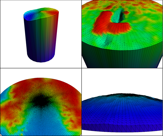
The illustration shows a spherical cap terrain model for a station poorly located on the edge of an open-pit mine. The pit is clearly seen in the zone B model. The zone D model is scaled to show the spherical curvature of the model. Top left panel: Zone A (166 m approx.) True scale. Top right panel: Zone A-B (1666 m approx.) 4x vertical exaggeration. Bottom left panel: Zone A-C (16666 m approx.) True scale. Bottom right panel: Zone A-D (166735 m) 10x vertical exaggeration.

The image below shows a spherical plate model, centred on Kangaroo Island in South Australia with 10X vertical exaggeration. We are viewing the model from above and to the East. The Datum level is 0m, so no bathymetry model has been generated. The crustal model is broken into multiple closed polyhedral and shows Kangaroo Island as well as the peninsulas in South Australia.

The next image shows the same spherical plate model of Kangaroo Island, now with a Datum level of -6000m. The crustal model now includes the continental shelf slope, right down to the abyssal plain. You can get a sense of the scale of the bathymetric terrain compared to the onshore terrain in this image.

The next image shows the same model, now looking up from below and to the west. Now we are visualizing the water model. You can see the island and the peninsulas now appear as holes in the model. The water column is shallow on the continental shelf but deepens rapidly as it follows the bathymetry of the continental slope and abyssal plain. The water model and the crustal model complement each other.

Products

All gravitation data is output in µms-2 units. Terrain height is expressed in metres, positive above sea level and negative below sea level. All model parameters are expressed in metres. The density of rock and water must be specified in g/cc. Sea level and the Datum level must be expressed in metres. The software generates the following outputs, depending on whether you choose to generate a flat Plate or a curved Cap or both.

TSP         Theoretical Spherical Plate

MSP       Modelled Spherical Plate (no terrain)

LSP         Modelled Spherical Plate, Rock (terrain and bathymetry to the datum level)

WSP       Modelled Spherical Plate, Water (bathymetry to sea level)

CSP        Complete Spherical Plate (LSP + CSP)

TCP        Complete Spherical Plate Terrain Correction (MSP – CSP)

TSC         Theoretical Spherical Cap

MSC       Modelled Spherical Cap (no terrain)

LSC         Modelled Spherical Cap, Rock (terrain and bathymetry to the datum level)

WSC       Modelled Spherical Cap, Water (bathymetry to sea level)

CSC        Complete Spherical Cap (LSC + WSC)

TCC        Complete Spherical Cap Terrain Correction (MSC – CSC)

Error     

RL           Land

RL           Bathymetry

It will generate the same set of outputs for each Zone, if requested. It will output 3D models for visualization, if requested. The Theoretical Plate and Cap calculations use analytic formulas. All other outputs are from 3D polyhedron models.

We supply an error code for each processed station. If no error was detected the code is zero but otherwise it will be a numerical combination of one of more of the following flags –

1              Slope of one or more inner ring petals of radius PR exceeds PA degrees.

2              Mismatch between the gravity and terrain elevation exceeds PR*cos(PA).

4              Terrain height – gravity station difference exceeds TZ within a radius of RZ.

The parameters that trigger these errors are based on criteria defined by Geoscience Australia and developed as quality control measures for survey operations. The radius of the inner petals (PR) is defined as the outer radius of Hammer zone B, equivalent to 16.6m. The maximum slope (PA) defaults to 5.0 degrees. The radius (RZ) is defined as Hammer zone C, equivalent to 53.3m, and the terrain tolerance (TZ) defaults to 20m.

Examples

Having prepared the software, it can be instructive and fun to use it to examine theoretical scenarios where terrain effects might be contrary to expectation and to explore bathymetry effects. I hope you find them instructive and I welcome any feedback by email. If you would like to use this software to process gravity observations, please contact me to discuss. You can download a PDF of this article here.

References

1. Argast, D. et al, 2009, An extension of the closed-form solution for the gravity curvature (Bullard B) correction in the marine and airborne cases: 20^th International Geophysical Conference
2. Barnett, C. T., 1976, Theoretical modeling of the magnetic and gravitational fields of an arbitrarily shaped three-dimensional body: Geophysics; v. 41; no. 6; p. 1353-1364
3. Blakely, R. J., 1995, Potential Theory in Gravity and Magnetic Applications: Cambridge University Press
4. Bullard, E. C., 1936, Gravity measurements in East Africa: Phil. Trans. Roy. Soc. London, 235, 486–497
5. Dentith, M., Mudge, S. Geophysics for the mineral exploration geologist: Cambridge University Press 2014
6. Hammer, S., 1939, Terrain corrections for gravimeter stations: Geophysics, v. 4,p. 184–194
7. Kirby, J., Featherstone, W., 2002, High-resolution grids of gravimetric terrain correction and complete Bouguer corrections over Australia: Exploration Geophysics, v. 33, p. 161-165
8. Lemoine, F. G. et al, 1998, EGM96: The NASA GSFC and NIMA Joint Geopotential Model, available from http://cddis.nasa.gov/926/egm96/egm96.html
9. Nowell, D.A.G., 1999. Gravity terrain corrections – an overview. Journal of Applied Geophysics, 42, 117-134.
10. 2007, Numerical Recipes: The Art of Scientific Computing, 3^rd edition: Cambridge University Press
11. Talwani, M., 1998, Errors in the total Bouguer reduction, GEOPHYSICS, VOL. 63, NO. 4; P. 1125–1130