Warrumbungles LiDAR Processing and Mapping

https://youtu.be/V9ZZPLKcz28?si=nP1wl8tvCs8IRy6q
https://youtu.be/M3knyapI-50?si=M9LoOZwnMp0xGj8h 

Introduction

The world was mapped by surveyors, and the results are accessible to everyone via Google Maps and similar webmap imagery. But new surveying techniques like LiDAR and photogrammetry are uncovering topographic features that traditional surveying overlooked. There are still things to be found out there!

ProRaster Scientific can be used to prepare high-resolution topographic maps that you can use when you are outdoors. I combine LiDAR ground surface grids with webmap topographic imagery to produce a map that is superior to Google Maps. These maps can be used when you don’t have internet data connectivity, or you can use them to identify and locate interesting topographic features.

Acquiring LiDAR data

LiDAR is a surveying technique that uses a laser to measure the separation between the airborne instrument and the topographic surface below. Each measured pulse-return is classified to record what the laser hit – trees, buildings, powerlines, the ground surface. A LiDAR survey produces a very large 3D point cloud which records position (XYZ) and classification as well as other parameters, often consisting of billions of points. By selecting the required returns by classification and gridding, you can turn a LiDAR survey into a high-resolution DEM.

There is a huge amount of publicly available LiDAR data available on government and private servers. When you acquire LiDAR data it will generally be in either a LAS or LAZ format. These formats are functionally equivalent, but LAZ files use lossless compression and consequently are cheaper to download and store.

Importing LiDAR

To consume LiDAR in ProRaster Scientific, you firstly import your LAS and LAZ files into an MRP file. An MRP file can contain a point cloud of unlimited size, and you can easily import thousands of LAS/LAZ files into an MRP.

On the Point Processing menu button, select “Import LiDAR > Import LiDAR…” to open the “LiDAR LAS/LAZ Import” dialog. For detailed information on how to use this dialog, see the ProRaster User Guide as well as YouTube video resources that guide you through the process.

https://youtu.be/Vy5_HN1Qdb8?si=tyvHG28FAlb0MN3C
https://youtu.be/ZLTovULvBms?si=t7SMDFAbNC-P2m42

There are three essential steps:

1. Select your LAS & LAZ files, either by browsing or by selecting all files of that type from a specified directory. You can add as many as you want, from as many directories as you want. As a rule, do not mix data from different LiDAR surveys. Use one MRP for one survey.
2. Make sure the coordinate system is correctly selected. This is usually obtained from the LAS/LAZ files automatically.
3. Specify the “Cell Size” from the MRP file. This will be proportional to the LiDAR point density. For older surveys a cell size of 1×1 metre might be suitable. For newer surveys that are higher resolution and higher point density, use a smaller cell size like 05×0.5 m or 0.25×0.25 m. It is a good idea to import a small fraction of the survey first to check your statistics to verify you have an appropriate cell size.

When you execute the import, your PC might hunker down for some time. It can take time and significant computing resources to import billions of points, spatially sort them, build overview levels, and compute high-quality statistics.

Once the MRP file has been generated, you can display it in any tier of ProRaster. You can color modulate the points by any parameter, and filter points for display by classification. Examine the statistics of the MRP file. Check what classifications are present (it varies and some surveys have not been classified at all).

Virtual gridding

Virtual gridding converts the billions of points in your MRP file into a gridded DEM at any scale in real time. You made ProRaster Scientific do the hard work when you created the MRP file – now you reap the rewards by being able to grid that data in real-time and examine it at any scale interactively.

On the Point Processing menu button, select “Virtual gridding > Virtual Grid…” to open the “Virtual Gridding” dialog. For detailed information on how to use this dialog, see the ProRaster User Guide as well as YouTube video resources that guide you through the process.

https://youtu.be/2_KgKOD6unw?si=9Y1helA9mBmx3cLJ
https://youtu.be/jh_YYt_erJA?si=L5Qm0hKD3-uQwfWF
https://youtu.be/MSe3KWS_A_k?si=-X2pUSogkmjBew_e
https://youtu.be/TcOeIg532-g?si=Kwypv5fOmULiHi9Z

There are two essential steps:

1. Select the MRP file you want to grid. If you want to combine multiple MRP files then create a Raster Source containing these MRP files, then select that. Specify the MVR output file (it is a small text file).
2. Choose the parameter you want to grid (like “Z”) and select a LAS Query to choose points based on classification and other parameters (like “Ground”).

Hit OK and your virtual grid will be displayed in a map. Zoom and pan to explore your data in real-time. You can display a virtual gid in any tier of ProRaster, but you can only create and edit an MVR in ProRaster Scientific. Edit an existing MVR by selecting it from the Point Processing > Virtual Gridding menu or just drag & drop the MVR onto ProRaster.

As your expertise with virtual gridding increases, you can experiment with different gridding techniques – triangulation and tensioned minimum curvature. Experts can employ “automated trend reinforcement” with tensioned minimum curvature to create the highest quality grids.

Exporting a virtual grid to MRR

If you are happy with the quality of your virtual grid and you plan to use it frequently, it can be useful to export the grid to a standard raster format. In ProRaster Scientific, select Export Raster from the Raster Processing menu button. Select the MVR file as the input, specify an MRR format raster as the output, and hit OK. MRR is the preferred format if you plan to use the raster in ProRaster. If you want to share the raster with users on other platforms, I suggest you export the MVR to MRR first then export the MRR to a standard format like GeoTIFF.

Building a topographic map

In ProRaster, you can now combine your high-resolution LiDAR DEM with other topographic map imagery. Your topographic imagery can come from any webmap source, like OpenStreetMap, Google etc.

Create a new algorithm from a webmap. This will generally add an Image layer to your algorithm. Connect the Intensity component to your DEM grid and enable it.

Tip: Right click on the map and Zoom to the extents of your DEM to ensure it is visible on screen.

Tip: The imagery will be clipped to the DEM by default, use the “Valid cell by component rule” setting in the layer properties to change this.

Adjust the intensity shadow and highlight parameters to get the right level of hill-shading.

Add a Contour layer, displayed above the webmap imagery, and connect the Color component to the DEM. In the Contour layer properties, you can adjust the contour levels, line color, line thickness and opacity, and labels.

Now you have a basic topographic map, but you can experiment with other techniques. For example, you can blend two or more webmap layers together. For example, you might combine Google Imagery with OpenStreetMap. Experiment with layer color processing to lighten dark areas in the imagery. Experiment with blending, and opacity modulation. Use the Calculator operation on the Raster Processing menu button to convert color webmap imagery to greyscale and opacity modulate by greyscale. Try using webmap overlay layers as an alternative.

Exporting a map to XYZ tiles

To get your topographic map into the field, ProRaster Premium and ProRaster Scientific provides an ability to export imagery out to a format called “XYZ OGC WMTS Tiles”. This is a multiresolution format and is used by all the major webmap providers (Google, Bing, OpenStreetMap etc). Make sure you name your algorithm and save it prior to exporting.

In ProRaster Scientific, select Export Image from the Raster Processing menu button. Select “XYZ OGC WMTS Tiles” in the Output Format dop list. At this stage, ProRaster will check that your algorithm is in the correct coordinate system. It must use EPSG 3857 (Projections of the World, Popular Visualization CRS). If required, change the algorithm coordinate system. (You can also choose “HandyGPS Offline Map” as an output format which produces the same output). Create and then select an empty folder into which the output will be written. The output consists of multiple sub-folders containing many small image files in PNG format.

You will probably need to clip the output to either the current extent of the map (in which case you ought to zoom it carefully before opening the Export Image dialog) or to a polygon.

Tip: You can draw your own polygon using the “Area” map tool and then exporting it to a polygon file.

Carefully choose the output resolution level, which determines the cell size of the highest resolution level. ProRaster gives you an indication of the size of the output raster and the true cell size (measured on the Earth). When you are ready, hit the “Process” button and ProRaster will generate the image files for each resolution level.

HandyGPS

When I am bushwalking, I navigate using an app on my phone called “HandyGPS” from BinaryEarth. HandyGPS allows you to display offline maps instead of, or in addition to, Google maps. You can use the XYZ Tiles you have generated in ProRaster Scientific as offline maps in HandyGPS.

The easiest way to do get your map into HandyGPS is to add all the files to a ZIP file, copy this to your phone, then direct HandyGPS to unzip and connect to it. In File Explorer, right-click on the output folder you created for the maps and select “Compress to… ZIP file”. Connect your phone to your PC and enable file transfers, then copy the ZIP file to the Downloads folder on your phone. In HandyGPS, go to the Map display and select “Manage offline maps…” from the menu. Hit “Import map from zip” and choose the ZIP file you created. HandyGPS will unzip the file and connect to the map. Thereafter you can easily change to this offline map or others you have created from the same controls.

https://www.binaryearth.net/HandyGPS/index.php

Exploring the Warrumbungles National Park

A Fat Man Off-Pissed in the Warrumbungles – Part 1 & 2

https://youtu.be/TwCERcZb7fE?si=BPANYltlOo0Pb1eT
https://youtu.be/TwCERcZb7fE?si=BPANYltlOo0Pb1eT

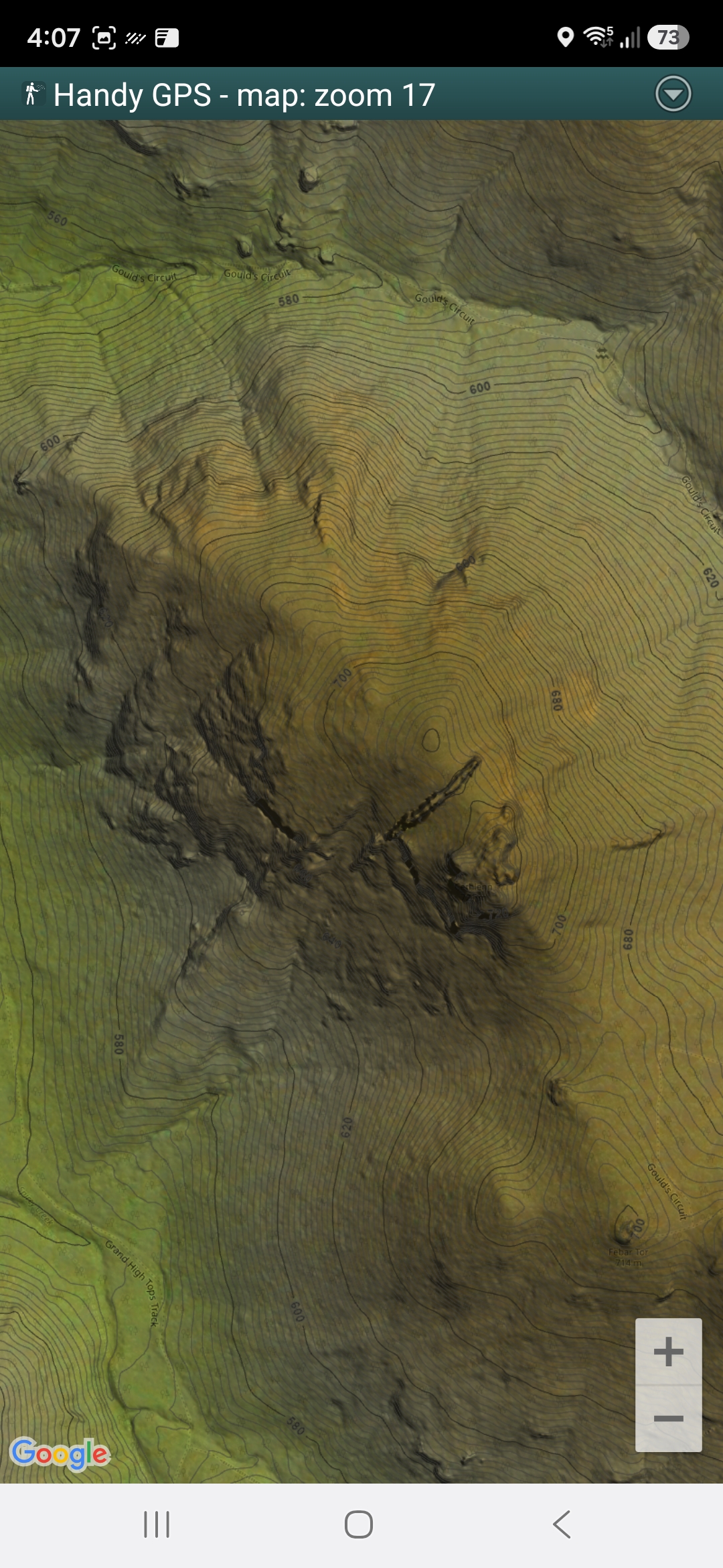
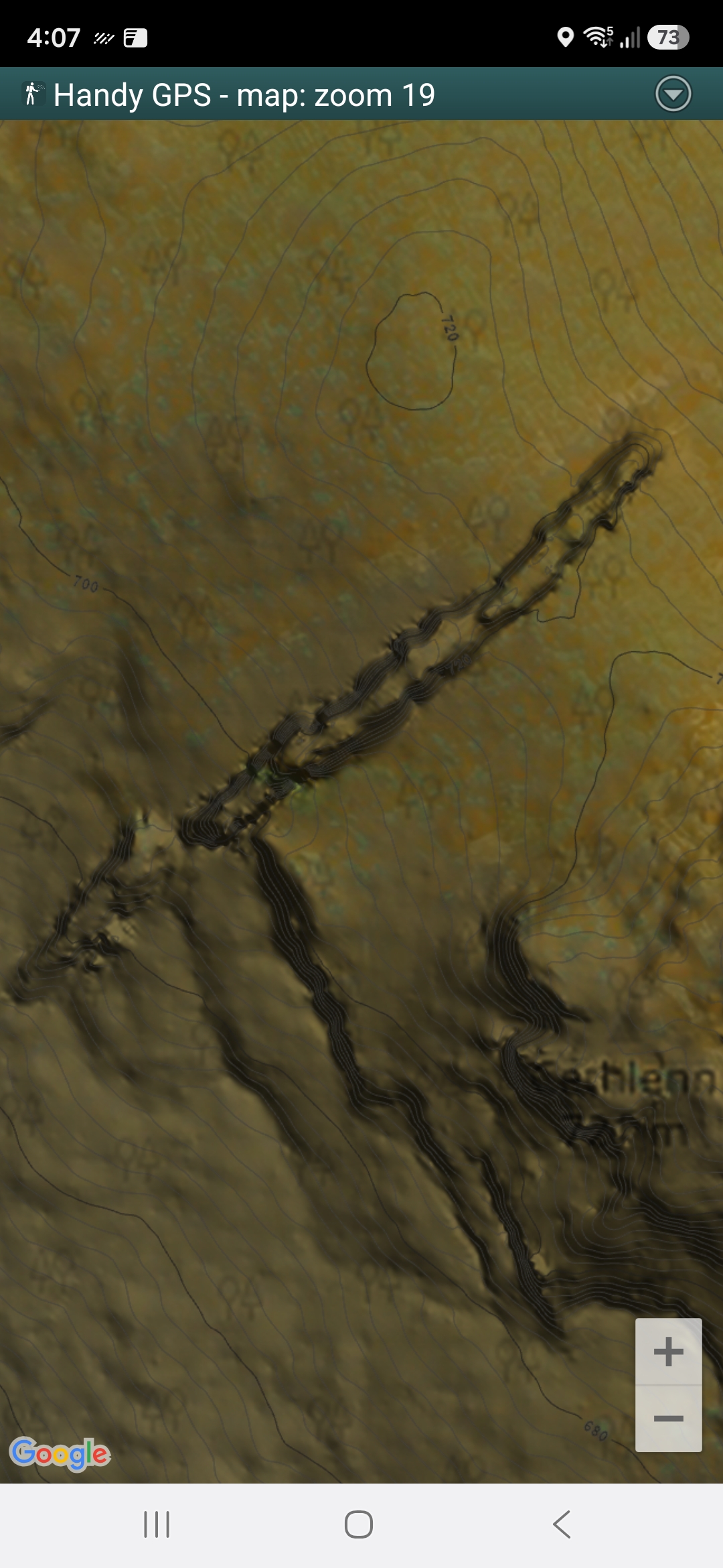
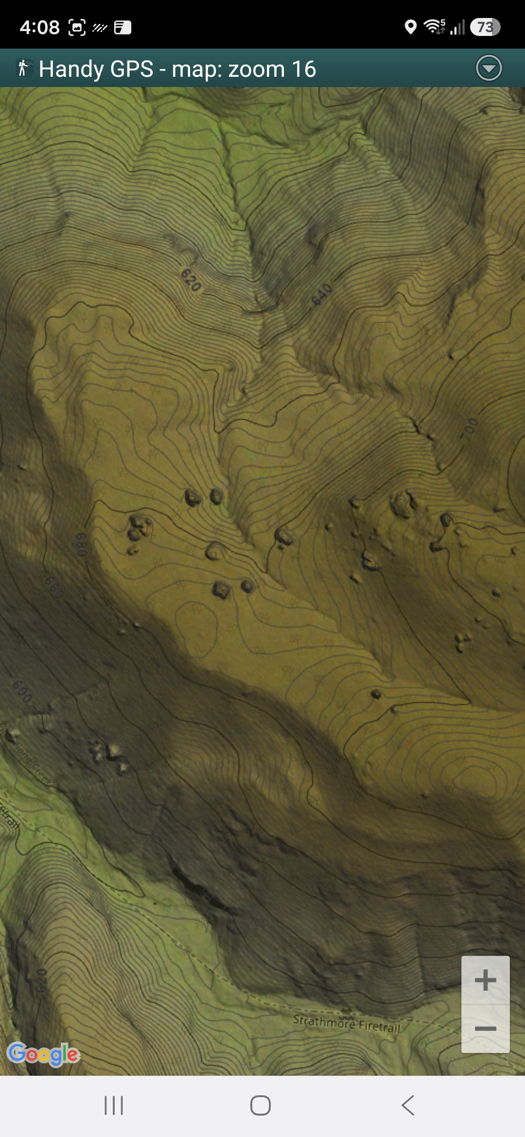
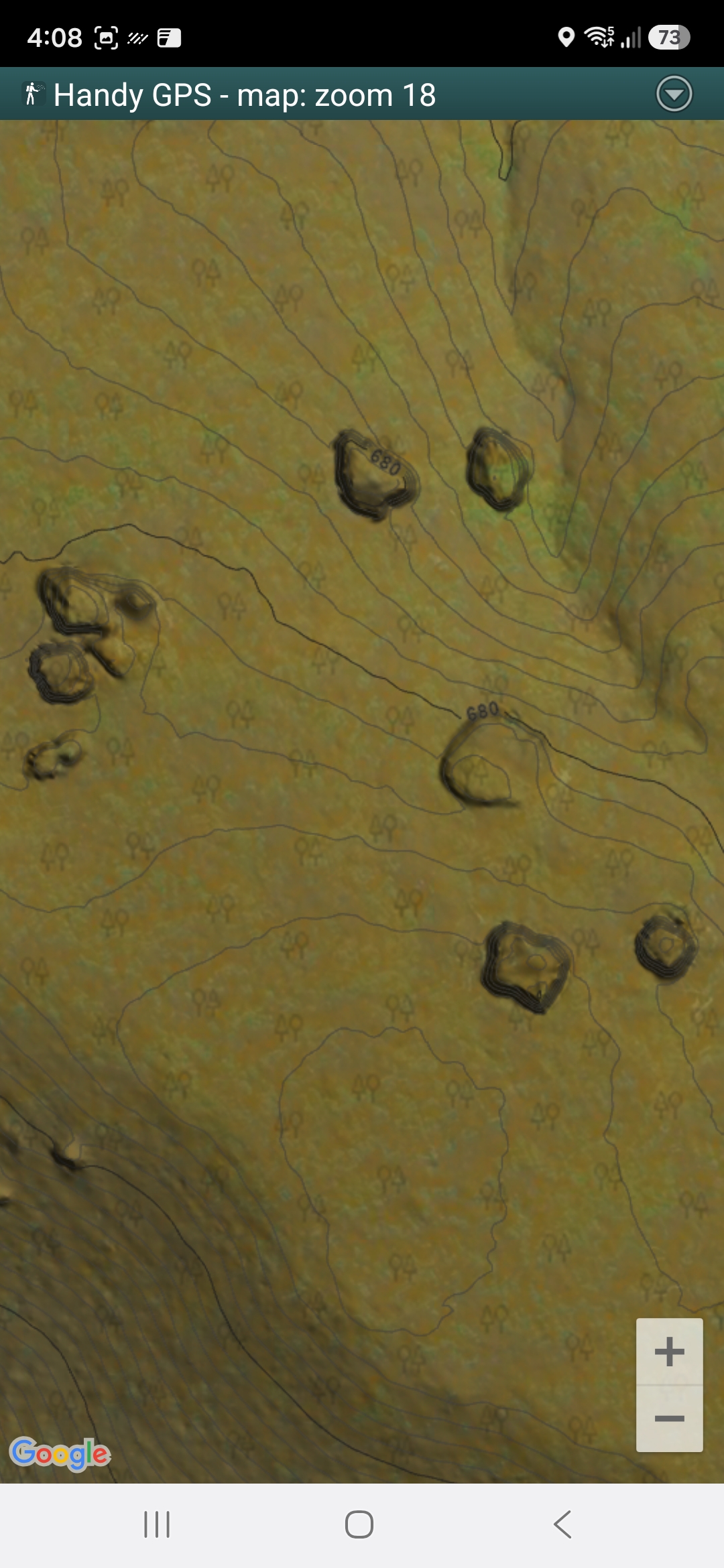
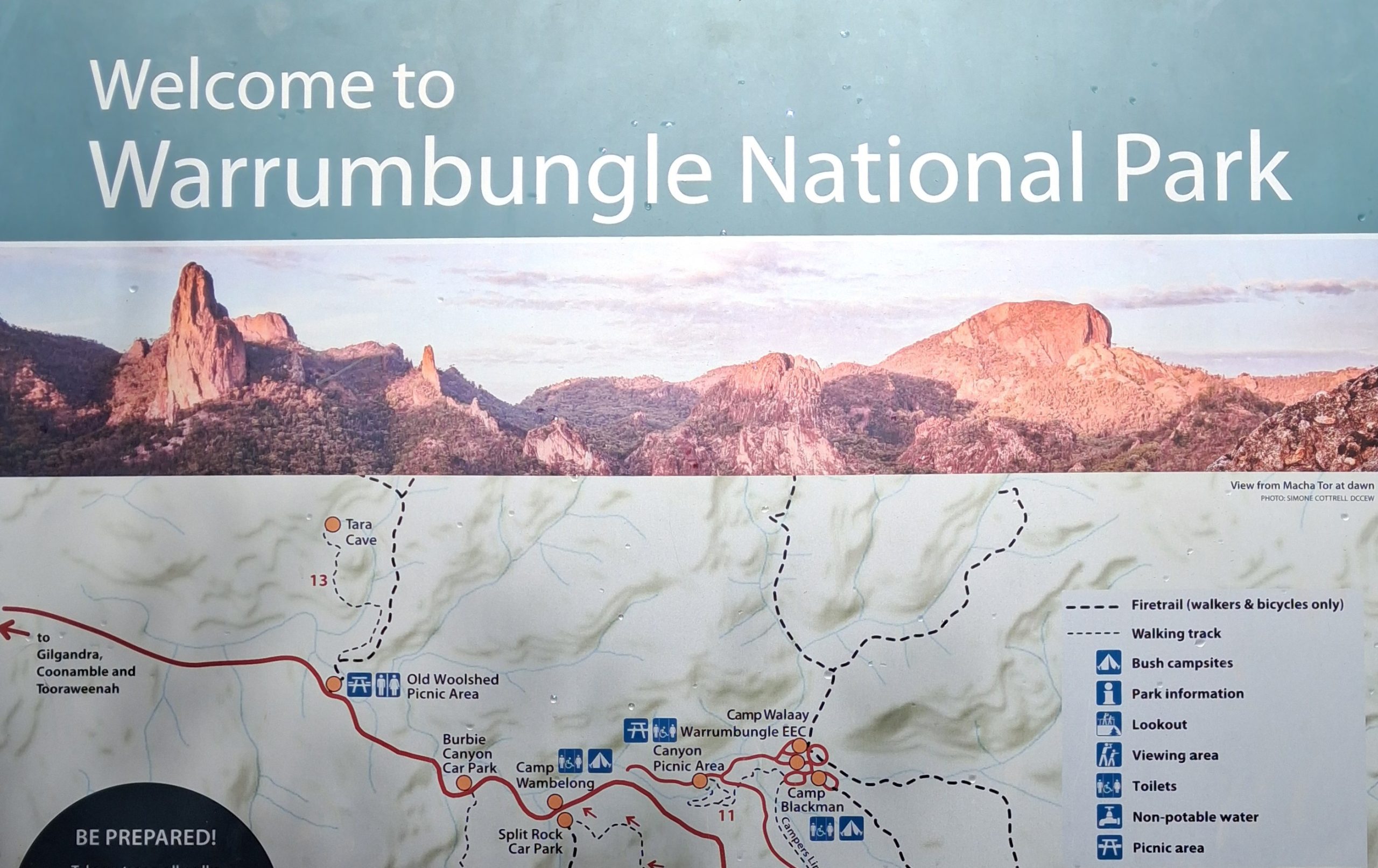
I prepared offline topographic maps for the Warrumbungles National Park in Australia. The LiDAR DEM showed interesting topographic features that were off the walking trails, and I visited two of these features. The first was a significant outcropping dolerite dyke crossing the peak of a hill (the Spinosaurus Sail), and the second was a collection of large, isolated boulders lying on a mountain terrace (the Wombat Bricks).

I created two offline maps, tightly clipped to polygons covering the intended day-walk. The maps combined LiDAR DTM as hill shading and contours with Google Imagery and OpenStreetMap. The maps were high enough resolution to enable me to identify individual boulders alongside the route as I proceeded.

The dyke is, perhaps, the second or third largest outcropping dyke in the park, and the second highest (the largest and highest being the Breadknife, a popular tourist attraction). It is exposed over a strike length of 95 metres and is up to 20 metres high.

The boulders are isolated, large, squarish monoliths, up to 15 metres high or more. They are 10 to 15 metres wide typically and in total there are about a dozen. Geological maps report that the country rock is Mount Naman Formation (porphyritic to equigranular trachyte to rhyolite lava deposits and intrusions) and I assume the boulders are of the same formation.

The Warrumbungles provide many good rock-climbing opportunities, and both topographic features described expand those opportunities. They are not big walls (like Belougery Spire or Bluff Mountain), but they would provide climbers with interesting top-rope climbs and bouldering.