

ProRaster Scientific
Welcome to the ProRaster Scientific product page!
Please download the feature sheet, the product guide, and the comprehensive user guide to learn about the product.
For the latest updates to ProRaster Scientific, please visit the Product Updates page. To see what is coming and to contribute ideas, visit the roadmap page.

You can safely and securely purchase and download ProRaster Scientific from the Microsoft Store. Read about the advantages of purchasing apps on the Microsoft Store. Hit the “Get it” button and you will be taken to the Microsoft Store where you can purchase and download the software.
Alternatively, follow this link to the ProRaster Scientific store website and from there you can access the Microsoft Store. Or, simply open the Microsoft Store on your PC and search for “ProRaster Scientific”.
You can install ProRaster Scientific for a free trial period of 7 days! Make the most of this opportunity and make sure the data you want to experiment and test with is to hand before you install the application and start your free trial. After the trial period ends you can return to the Microsoft Store to purchase the product if you wish.
Please make sure it is compatible with the multispectral data you wish to view and analyse, and that your requirements will be met working within the limitations of the product.
Thank you for purchasing ProRaster Scientific! You are now a part of the ProRaster team. Please drop us a note via the contact page, we would love to hear from you. Please report bugs and suggestions, we welcome your feedback.
Rendering features at an glance

LUT Color Layers
Color modulate any gridded raster data and apply intensity shading and specular highlights. Aeromagnetic Data with Street Maps Overlay.

LUT Color Layer Blending
Blend multiple layers of any type together to build rich renderings. LiDAR-derived Terrain and Bathymetry blended with Tree Canopy Height.

RGB Color Layers
Combine color modulated red, green, and blue color components and apply intensity shading and specular highlights. Potassium – Thorium – Uranium tri-color radiometric data, hill-shaded by terrain.

Image Layers
Display imagery of any size, opacity modulated, and apply intensity shading and specular highlights. UK Ordnance Survey Topographic Imagery, hill-shaded by terrain.

Classified Rasters
Render classified (thematic) rasters using any layer type. Land use raster, hill-shaded by terrain. Spreadsheet data tracking mouse cursor.

Contour Layers
World’s best real-time contouring of rasters of any size or scale. Mt Kilimanjaro, GLO-30 terrain. LUT Color and Contour layers.

Rich multi-layered algorithms
Blend and overlay layers to build up information-rich imagery. Colored terrain blended with Google Maps imagery, OpenStreetMaps overlay, and terrain contours, Mt Fuji.

3D maps driven from 2D map zoom and extent
Display multiple 3D surfaces in one or more 3D maps. LiDAR-derived Terrain and Bathymetry and Tree Canopy Height.

Interactive 3D Maps
Fly and navigate about multiple 3D surfaces in one or more 3D maps. Supports high-performance rendering of high depth-complexity transparent surfaces. LiDAR-derived Terrain and Bathymetry and Tree Canopy Height.

WebMap WMS/WMTS
Ships with a collection of ready-to-use WebMaps, or connect to other WMS/WMTS sources. Mt Etna, OpenStreetMaps imagery hill-shaded by terrain, contoured.

WebMap Overlays
Overlay real-time modified street map data on raster imagery to preserve the underlying layer colors and saturation. OpenStreetMaps on Land Use classified data.

Interactive Profile Tool
Draw or import polylines and interactively extract raster profiles at any scale. Save and export. Mt Kilimanjaro GLO-30 terrain profiles.

Image Swapping Layer and Group Comparison Tool
GEBCO 2024 (left) being compared to GLO-30 (right) using the horizontal slider tool.

Image Swapping
Compare layers and groups of layers using the swapper tool. Comparing aeromagnetic data with mapped geology.
Earth Observation Imagery features at an glance

Satellite Multispectral Earth Observation Imagery
Sentinel-2C Surface Reflectance (Bottom of Atmosphere) True Color RGB Layer. Push scenes and tiles from the MSS Scene Browser into the rendering interface.

Satellite Multispectral Spectral Index
Render scores of in-built spectral indices. Sentinel-2C Surface Reflectance (BOA) derived Normalised Difference Vegetation Index (NDVI).

Landsat Scene Mosaic
Create a wide variety of advanced multispectral Products from scenes and tiles. Apply processing and analysis operations. Landsat Mosaic, Kati-Thanda, Australia.

Multispectral Product Editor
Build waterfall style cascading virtual processing chains, ending in rendering and analysis.

Pakistan Flood 2022
Analysis of the extent of the flooding in Pakistan, 2022. Landsat 8 & 9.

NDVI Spectral Index
NDVI vegetation index, clipped to cropping lands classification. Murray River.

Earth Observation Imagery.
Render and enhance band combination. Ocean and Land using different band combinations. Sentinel-2, Northern Australia.

Pansharpened Landsat
Apply pan-sharpening in real-time to Landsat.
Processing features at an glance

Export your Imagery
Export your algorithm imagery – covering any region, or clipped to any polygon – at any resolution. No limits. GEBCO 2024, clipped to Australia, GeoTIFF output.

Virtual Processing Operations
Apply processing operations on huge rasters with just-in-time computation. Calculator operation rendered, contoured, and profiled, GLO30-MERIT DEM, Mt Everest region.
Point Cloud Processing features at an glance
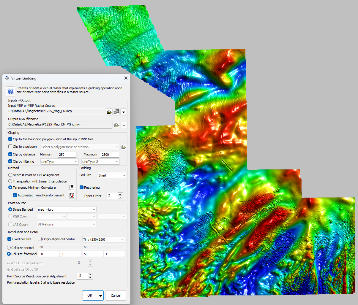
Virtual Gridding Aeromagnetic Survey Data
Line-based magnetic intensity data gridded in real-time using tensioned minimum curvature
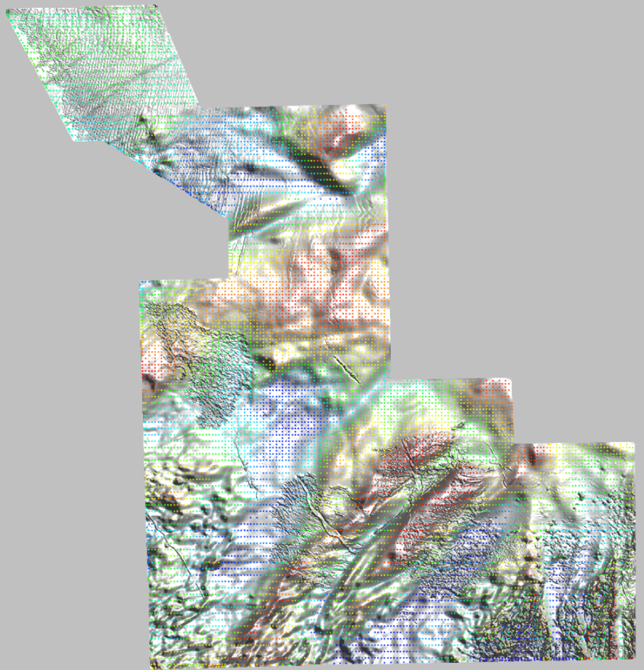
Point Display and Virtual Gridding Aeromagnetic Survey Data
Colorised point data displayed on top of magnetic intensity data gridded in real-time using tensioned minimum curvature
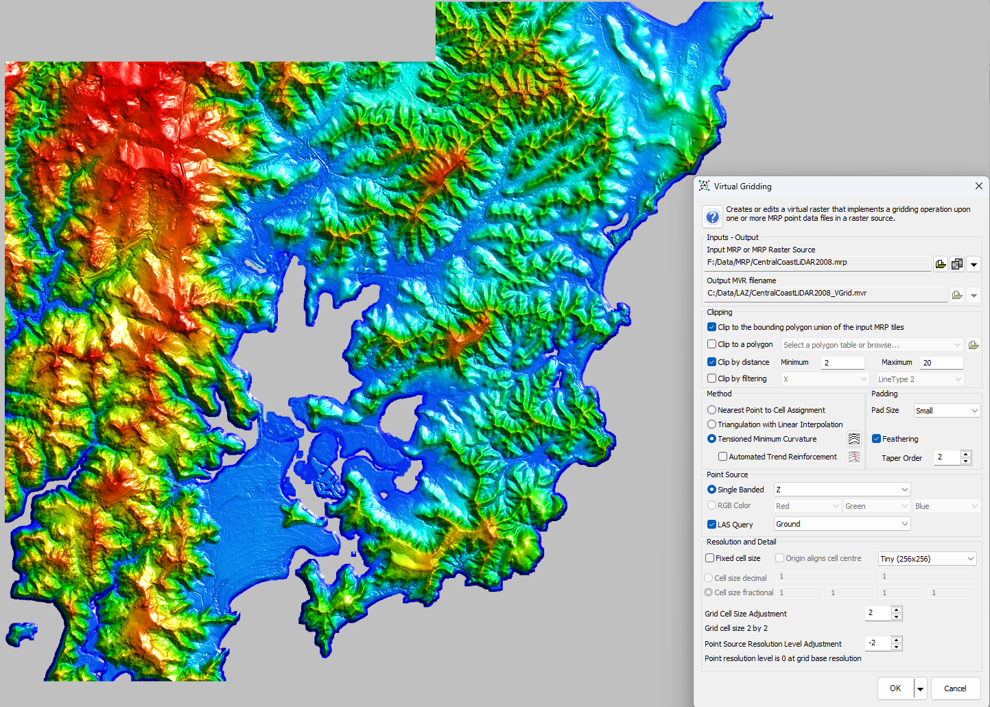
LIDAR Ground Returns Virtual Gridding in Real-Time
6 billion LIDAR ground returns gridded in real-time with tensioned minimum curvature.
What is ProRaster Scientific?
ProRaster Scientific is an advanced raster creation, processing, and rendering toolkit. The Point Cloud processing module imports LiDAR (LAS/LAZ) and Multi-banded Point data and generates virtual grids in real-time. The Earth Observation Imagery module provides specialist tools for rendering, processing, and analysing multispectral satellite imagery. The advanced virtual raster processing pipeline technology minimises time, costs, and computation resources, whilst maximising efficiency, performance, and data quality.
ProRaster Scientific delivers four major capabilities –
Raster rendering engine
Use the raster rendering engine to build and edit multilayered “rendering algorithms”. This class-leading capability transforms raster data into rich, beautiful, and informative imagery. The multi-threaded and hardware-accelerated rendering engine provides immersive imagery rendering that will help you make discoveries and maximise your understanding of the data.
ProRaster Scientific includes all the features of ProRaster Premium and ProRaster Essential.
Raster processing operations powered by virtual raster technology
Traditional raster processing imports a source raster and applies a processing operation to it, then exports an output raster. This process consumes time, computing resources and storage, and you can’t check the result of your processing operation until the output has been generated. ProRaster Scientific uses virtual raster technology to apply processing operations in real-time, at any scale, to rasters of any size. It takes no time, uses no resources, and the results can be rendered immediately allowing you to see if your processing operation has acted appropriately. The virtual raster output can be used as input to another operation, so you can build chains of processing operations. To take your data into other platforms, crystallise your virtual raster at any time by exporting it to a standard raster format like GeoTIFF or MRR.
ProRaster Scientific includes all the functionality of ProRaster Essential and ProRaster Premium.
Multispectral satellite imagery rendering, processing, and analysis, powered by virtual raster technology
ProRaster Scientific is a powerful and efficient platform that enables experts and amateurs to maximise their productivity when rendering, processing, and analysing multispectral satellite imagery. Chain together processing operations with advanced virtual raster technology to shepherd your imagery from the original rasters through to advanced derived products. Do less and achieve more – faster and more efficiently!
The fully automated import process applies corrections to your Landsat (1-9) or Sentinel2 imagery scenes and builds pixel masks from QA data. Graphically and spatially query your scene database to select scenes from which to create new multispectral imagery products. Your product may combine imagery spatially (mosaics), temporally (sequences), by pixel compositing (collating – masking out bad quality pixels and back-filling with high-quality pixels from temporally adjacent imagery), or by a combination of these concepts.
A multispectral imagery product, regardless of its complexity or dimensionality, is a single virtual raster. Now, using the graphical product editor, chain together processing operations to operate on your product. Typically, you will apply pixel masking to remove clouds, then choose from more than 100 spectral indices that help quantify vegetation characteristics, map surface water or fire scars, measure soil moisture, and much more. Apply calculator operations and non-linear data transformations, if required, and focus on a region of interest by clipping to a polygon. Complete your analysis by computing multidimensional statistics, rendering imagery and spectral indices, and batch exporting imagery for video production.
Point Cloud Import, Processing, and Virtual Gridding
ProRaster Scientific can import multi-banded point datasets into a new storage file format called MRP. This sparse tiled point storage format spatially sorts and indexes point data, creates and stores overview resolution levels, and computes and stores comprehensive statistics.
ProRaster can import LiDAR data from LAS or LAZ source files into an MRP file. The full LiDAR pulse-return data structure is duplicated in the MRP. Users can then design LAS Queries to extract desired returns for rendering or gridding in real-time.
ProRaster can display point clouds stored in MRP files. Use LUT or RGB color modulation, opacity modulation, and masking. Apply a LAS Query to filter LiDAR returns in real time. Render an unlimited number of points in real-time, only bounded by your storage capacity.
ProRaster can grid point clouds in real-time using a virtual gridding operation. This remarkable capability allows you to grid and render trillion-point datasets in real-time, at any scale. Interactively modify your gridding method parameters to control the gridding operation. Select from Nearest Neighbour, Delauney Triangulation, or Tensioned Minimum Curvature gridding methods.
ProRaster provides a unique extension to the Tensioned Minimum Curvature gridding method that applies Automated Trend Reinforcement in real-time. The algorithm analyses the data to identify the dominant trend direction at every pixel and then applies a bias to the minimum curvature interpolation to reinforce that trend direction. The result is an extraordinary improvement in raster quality and continuity.
How does Multispectral Imagery Processing Work?
ProRaster Scientific has automated support for all Landsat imagery and Sentinel2 imagery, and manual support for other platforms. It uses the power of virtual rasters to eliminate data duplication and maximise processing efficiency, saving you time and money.
To get started with multispectral imagery in ProRaster Scientific, you will follow a processing pipeline like this –
1. Download scenes or tiles from your data provider.
The Earth Observing Satellites acquire data in swaths called a “scene”. Each scene covers a static footprint on the Earth and the satellite will typically revisit that scene regularly and reacquire it many times over the life of the bird. This data is processed and then distributed to users as a package containing rasters for each spectral band and other information. This is a scene, and it is your starting point. A tile is a rectangular subset of a scene.
You can download Landsat scenes for free from USGS Earth Explorer –
https://earthexplorer.usgs.gov/
You can download Sentinel 2 tiles for free from the Copernicus Browser accessed via the Copernicus Data Space Ecosystem –
https://dataspace.copernicus.eu/
2. Unpack and store your scenes on your local drive or network.
The scene/tile will be delivered as a compressed archive. You will need to decompress (unpack) this archive and store the data package on your local drive or network. How you organise this is up to you.
The data package generally consists of multiple rasters, each of which contains observational data over a spectral frequency range, as well as other ancillary rasters. It can be difficult to know what files correspond to what spectral bands, but ProRaster takes care of those details for you.
3. Create a multispectral scene database and add the scenes to the database.
In ProRaster, add each scene/tile you download to your scene database. The database is a small file that links to the original raster data – it does not contain a copy of the raster data. ProRaster will generate a “scene assembly virtual raster” for each new scene/tile and store it alongside the database. You will access all data from the scene via this assembly MVR from now on.
The scene assembly MVR will apply all the corrections required to translate the raw digital numbers supplied to reflectance.
4. Render the scenes.
Take a look at your new scene! Open the scene database browser and select the scene. Right-click and from the pop-up context menu, select “Render Scene”. Choose a band combination to highlight specific attributes of the Earth. A rendering algorithm will be created for your scene in the main ProRaster interface, and the scene will be displayed in a map.
5. Create a multispectral product database.
In ProRaster we distinguish between a basic scene and a multispectral data product. A product starts life as one or more scenes, to which you can apply processing operations in a waterfall cascade pattern. Before you can create a product, you need to create a database to store it in.
6. Browse for and select scenes from which to create a multispectral product.
Open a scene database browser and select a scene. Right-click and from the pop-up context menu, select “Create scene product”. A new product will be added to your product database and the new product will be opened in the product editor dialog.
7. Edit the product and apply processing operations.
You can apply a growing list of processing operations to the scene in your product including – Mask, Clip, Index, Reproject, Calculator, Transform, and Difference. You can generate a rendering algorithm, compute statistics, and export the data to a raster. Define these operations in any order you wish to build a waterfall cascade processing pattern. Thereafter, when you change any operation, all the downstream operations will get updated.
As your level of expertise improves, you will go on to combine products into more advanced products and combine rendering algorithms into more advanced visualisations. Soon, you will be using the “Create Product Sequence Wizard” to build advanced temporal sequence (multidimensional) products.
How does Raster Processing work?
Traditional raster processing imports a source raster and applies a processing operation to it, then exports an output raster. This process consumes time, computing resources and storage, and you can’t check the result of your processing operation until the output has been generated.
ProRaster Scientific takes a different approach. It uses virtual raster technology to apply processing operations in real-time, at any scale, to rasters of any size. It takes no time, uses no resources, and the results can be rendered immediately allowing you to see if your processing operation has acted appropriately.
As an example, consider a very large gigapixel scale raster. If you were to clip this raster to a polygon and output a new raster it might takes minutes or hours to execute the processing. But in ProRaster we simply create a virtual raster (which takes no time and uses no resources) then immediately render it. The clipping occurs in real-time as you render the raster.
Furthermore, the virtual rasters we create as output from each operation can be used as input to another operation, so you can build chains of processing operations. The multispectral product editor leverages this technology.
To take your data into other platforms, crystallise your virtual raster at any time by exporting it to a standard raster format like GeoTIFF or MRR.
How does Raster Rendering work?
All raster data is rendered in ProRaster by building a rendering algorithm. A rendering algorithm can be saved to disk as an MRD file. If you take a look at one, you will find it just contains standard XML.
The rendering engine in ProRaster takes a rendering algorithm and, following the instructions therein, converts the raster data to colored pixels. It uses multithreading and hardware graphics acceleration to get those pixels into your map as quickly as possible for immersive, fluid rendering.
The rendering engine is laser-focused on outputting the highest quality imagery at all times. You do not have to worry about raster cell size, cell alignments, coordinate systems, or data interpolation. Give it any raster data, in any combination, with any properties, and it will give you pixel-perfect imagery every time.
Here is a high level overview of rendering algorithm capabilities –
- Create, load, and edit rendering algorithms and save to MRD format.
- Combine multiple Image, LUT Color, RGB Color, Contour, and 3D Surface layers.
- Image layers combine RGB(A) or Greyscale Imagery with Intensity modulation, Opacity modulation, and Pixel Masking components.
- Color LUT layers combine a Color component (which maps data values into a color lookup table) with Intensity modulation, Opacity modulation, and Pixel Masking components.
- RGB Color layers combine Red, Green, and Blue components (which map data values to color) with Pan-sharpening, Intensity modulation, Opacity modulation, and Pixel Masking components.
- Contour layers render the world’s highest-quality contours in real-time, with Opacity modulation and Pixel Masking components.
- 3D Surface layers define a geometry surface for rendering algorithms in 3D maps.
- Manage your Color Table, Data Transform, Data Conditioning Filter, and Raster Source global resources through comprehensive editors.
- Map Tools help you explore and compare rasters. Distance and Area measurement, Interactive Profiles, and Layer and Group image Swapping.
How does Point Cloud Import and Virtual Gridding Work?
Point data is supported in ProRaster Scientific with these capabilities –
- A new file format called “MRP” for storing multi-banded 2D point data and LiDAR 2D pulse-return data.
- An import operation for multi-banded 2D point data that supports creating new MRP files and adding new data to existing MRP files.
- An import operation for 2D LiDAR pulse-return data that supports creating new MRP files and adding new data to existing MRP files.
- Support for rendering points (stored in one or more MRP files) in the main rendering interface. This capability is shipped with all tiers of ProRaster.
- A Virtual Gridding Operation that will grid point data stored in one or more MRP files in real-time and allows users to interactively modify gridding parameters on-the-fly.
- A global resource editor, the LAS Query Editor, that enables users to create and edit queries that acquire returns from LiDAR pulse-return data. These queries can be employed when rendering and gridding LiDAR pulse return data stored in an MRP file.
MRP is a new point cloud file format that provides efficient storage of 2D point cloud data.
- MRP supports datasets of unlimited size and addresses the problem of huge point cloud management by minimising storage requirements through sparse tiled storage, rich type selection, and efficient lossless data compression.
- MRP supports high-performance access – and constant time access – to point cloud data at any scale by generating a data pyramid of overview resolution levels that are stored within the MRP file.
- MRP supports the temporal dimension.
- An MRP file is editable and extensible. Additional compatible point cloud data can be added to an existing time event, or as a new time event.
- An MRP file spatially sorts and indexes data in 2D (using the designated X and Y coordinate bands).
- An MRP file contains comprehensive summary statistics for all data bands.
MRP files come in two flavours – general Multi-banded point cloud files, and LiDAR pulse-return files.
- A general multi-banded point cloud MRP (PNT_MRP) can contain any point data, with the expectation that bands for X and Y coordinates will be supplied as a minimum requirement.
- A LiDAR pulse-return point cloud MRP (LAS_MRP) contains LiDAR data imported from LAS or LAZ files.
ProRaster takes a different approach to point data management, gridding, and processing to other software. The end-goal is to grid huge point datasets in real-time and enable visualisation and analysis of gridded point data without enormous pre-processing operations. To achieve this, you must first import your point data into an MRP file. (Note that this creates a new “hardcopy” duplicate of your point data). Once in MRP format you will be able to render, grid, and process point datasets in real-time at any scale.
The ProRaster point cloud data processing pipeline looks like this –
- Import raw point data into an MRP file.
- Import multi-banded point data to a PNT_MRP or –
- Import LiDAR (LAS/LAZ files) pulse-return data to a LAS_ MRP.
- Add to and extend an existing MRP spatially (or temporally) by importing new data of the same type.
- Render the MRP file in ProRaster to inspect and validate point data.
- Undertake visual and statistical quality control.
- Color modulate points by using either a LUT Color style data-color transform or an RGB Color style data -color transform. Color tables are included for rendering LAS_MRP data by classification code.
- Apply a LAS Query to LAS_MRP data on-the-fly to filter and select returns.
- Use tooltip reporting in the map to reflect the value of any point as you pass over it with the mouse cursor and display the value of all bands using the “Key + Table” reporting option.
- Employ Virtual Gridding to transform the point data into a continuous raster in real-time at any scale.
- Grid point datasets of unlimited size down to very high resolution.
- Modify your gridding method and gridding parameters interactively and see this reflected in the gridded raster in real-time.
- Apply a LAS Query (which you can change at any time) to LAS_MRP data to select returns for gridding.
- Render the virtual grid (in 2D, 3D, as imagery or contours) to explore your data and undertake QC inspection.
- Use the virtual grid as input to any other virtual processing operation or chain of operations (for example Clip to a polygon and apply a Calculator operation).
Basic Training
The following videos are best viewed on YouTube and will help you learn how to use ProRaser Scientific. Don’t forget to “like and subscribe” and if you leave a comment or question, we will be able to respond to it.
ProRaster Scientific 2.4.01 – 3D Maps Deep Dive Tutorial
ProRaster Scientific version 2.4.01 supports 3D maps in which you can display one or more 3D surfaces draped with imagery, directly from your 2D rendering algorithm. Take a deep dive into 3D surface rendering and learn how to use this feature in ProRaster Scientific.
Classify Raster Processing Operation
See how to use the new Classify (raster) processing operation in ProRaster Scientific 2.2.09.
New User Interface Features
I take you on a walk-around of the new user interface features in ProRaster Scientific.
ProRaster Scientific builds on – and extends – ProRaster Premium. This video takes a quick look at the new user interface elements in ProRaster Scientific.
Downloading Landsat Scenes
I take you through the basics of downloading a Landsat scene from Earth Explorer and importing it into ProRaster Scientific.
Rendering Satellite Imagery
See all the different ways that you can render a multispectral satellite imagery scene in ProRaster Scientific.
I build algorithms manually, via the scene database browser, and via the product editor. There are many ways to render multispectral data in ProRaster Scientific and it is important to be familiar with the most efficient and powerful mechanisms.
The Multispectral Scene Database
Learn how to create and maintain multispectral satellite scene databases in ProRaster Scientific. See demonstrations of how to import scenes and find out what the scene database does, and where it is stored.
Using the Scene Database Browser
Learn how to use the multispectral satellite scene browser to query your scene database and find the scenes you want.
See how to create products from the browser including scenes, mosaics, collated scenes and mosaics, and scene sequences.
The Multispectral Product Database
Learn how to create and maintain multispectral satellite product databases in ProRaster Scientific. Find out what the product database does, and where it is stored. See how to make products from scenes and how to edit products.
The Multispectral Product Editor
Learn how to build virtual processing cascades in the multispectral satellite imagery product editor in ProRaster Scientific. See an overview of the operations available and learn how to control operation execution.
The Create Product Sequence Wizard
Learn how to turbocharge your productivity with the powerful new “Create Product Sequence” wizard in ProRaster Scientific version 2.2.
Working with Spot7 Imagery
Learn how to manually import a Spot7 multispectral satellite scene into ProRaster Scientific. With high-resolution Blue, Green, Red, and Near Infrared spectral bands, Spot7 data provide ample opportunity for vegetation analysis.
Working with GeoEye1 Imagery
Learn how to manually import a GeoEye1 multispectral satellite scene into ProRaster Scientific. With high-resolution Blue, Green, Red, and Near Infrared spectral bands and with a very high-resolution panchromatic band, GeoEye1 data provide ample opportunity for vegetation analysis.
Before watching this video, watch the Spot7 video which covers the procedure in more detail.
Introducing the Processing Menu
Explore the new Raster Processing operations in ProRaster Scientific. The operations generate virtual raster outputs and so operations on huge rasters can be visualized immediately, without executing any processing!
Worked Examples
The following videos are best viewed on YouTube and show how to use ProRaster Scientific in worked examples using real data and analysis.
Change Matrix Analysis of USA National Land Cover (Annual NLCD) using ProRaster Scientific
The Annual NLCD dataset is a collection of 40 land use classification rasters, providing temporal coverage from 1985 to 2024 for the USA. This video demonstrates how to use ProRaster Scientific to process these rasters to analyse land use change in the USA over 40 years. See examples of how to use the Classify Raster Operation, Export Raster Operation, Raster Time Sequence Operation, Time Differential Operation, and Change Matrix Operation in ProRaster Scientific.
Quantifying vegetation health at Macquarie Island before and after pest species eradication
I use freely available Landsat Earth Observation multispectral imagery and ProRaster Scientific to quantify vegetation health at Macquarie Island before and after a long-term pest species eradication program.
Located halfway between New Zealand and Antarctica, Macquarie Island is a cold and windswept haven for Southern Ocean sea birds, penguins, and marine mammals. A program has been conducted by Australian governments to eradicate pest species on the island including rabbits, rats, and mice. These pest species were degrading the island vegetation and impacting the breeding behaviour of resident and visiting wildlife.
I acquire Landsat 7 scenes from 1999-2002 and Landsat 8 & 9 scenes from 2022-2024 to compare NDVI (vegetation index) statistics before the eradication program and after it. The data show a stark improvement that testifies to the success of the program.
Preparing GLO-30 DEM Data in ProRaster Scientific
GLO-30 is a one-arcsecond (30 metre) resolution global DEM raster that can be acquired for free from the ESA via Copernicus. You can download 1×1 degree tiles in TIFF format as packages for countries and regions.
In the first video, I show you how to take the tile collection for a country and work with it in ProRaster Scientific. Firstly, I create raster sources for the DEM files and the WBM water mask files. Secondly, I use the “Create Raster Mask” operation to create a mask from the WBM files that retains pixels classified as Land, Rivers, and Lakes but removes Ocean. Thirdly, I use the “Clip to Raster” operation to clip the DEM to the Ocean mask. Finally, I export this virtual raster (MVR) to a physical raster (MRR). From almost 2.5 GB of original source data, I create a high-quality DEM raster in MRR format that only uses 26 MB – a 100x improvement in storage efficiency.
In the second video, I show you how to prepare the mask rasters using the Classify processing operation. These include the Height Error Mask, the Water Body Mask, the Filling Mask, and the Edit Data Mask.
Maping the 2022 Indus Valley Flood, Pakistan
I compute the area of Pakistan that was flood affected in the 2022 flood event in the Indus Valley. This was stimulated by a three-way comparison where experts used Google Earth Engine, Microsoft Planetary Computer, and QGIS to make this computation. As a result of this analysis, I added some new compositing features to ProRaster Scientific. In the second video, I use these new techniques to come to a final estimate of 27,772 square kilometres.
GEBCO 2023 Gridded Bathymetry Data in ProRaster Scientific
Each year GEBCO releases an updated bathymetry raster for the world at 15 arc second resolution. I download the eight TIFF files and show you how to display them in ProRaster Scientific. My first approach is to use the Raster Source Editor to create a raster source for the TIFF files. Then, I use a Join operation to create a virtual raster for this raster source. Finally, I export the virtual raster to an MRR format raster. I take a look at the bathymetry off the northwest coast of the Kimberly in Australia, then lower the sea level by 91 metres to reveal the paleo-topography of this region.
Coorabulka Revisited – NDVI Analysis
Taking advantage of new productivity tools in ProRaster Scientific version 2.2.03, I repeat the Coorabulka NDVI analysis in real time in a single video! We start with 552 Landsat 8 and Landsat 9 scenes, Collection 2 Level 1. I create a scene database, then use the Create Product Sequence Wizard to generate a Collated Mosaic Sequence product over more than 10 years. I then compute NDVI, clipping the data using a calculator expression, and clipping the raster spatially to the Coorabulka Station polygon. I compute statistics and then convert NDVI (Normalised Difference Vegetation Index) from a vegetation index to a proxy measure of “Feed On Offer” using a non-linear data transformation.
ProRaster Scientific NDVI Analysis – Coorabulka Station – Part 1 of 6
In this six-part series, I use ProRaster Scientific to perform a vegetation change analysis at Coorabulka Station in western Queensland over an entire year from July 2022 to July 2023. Coorabulka is located in the “channel country”, where infrequent flooding events can transform the station’s vegetation and carrying capacity.
In Part 1, I take a look at Coorabulka and the hardware I use to perform the processing, then build the multispectral satellite imagery scene database in ProRaster Scientific.
ProRaster Scientific NDVI Analysis – Coorabulka Station – Part 2 of 6
In this six-part series, I use ProRaster Scientific to perform a vegetation change analysis at Coorabulka Station in western Queensland over an entire year from July 2022 to July 2023. Coorabulka is located in the “channel country”, where infrequent flooding events can transform the station’s vegetation and carrying capacity.
In Part 2, I show you how to build mosaics from satellite scenes and then discuss the advantages of using collation to improve your data quality in a mosaic. We put these mosaic products together into a mosaic sequence that adds a temporal dimension to our raster dataset.
ProRaster Scientific NDVI Analysis – Coorabulka Station – Part 3 of 6
In this six-part series, I use ProRaster Scientific to perform a vegetation change analysis at Coorabulka Station in western Queensland over an entire year from July 2022 to July 2023. Coorabulka is located in the “channel country”, where infrequent flooding events can transform the station’s vegetation and carrying capacity.
In Part 3, we go deeper into building high-quality Collated Mosaic Sequences that draw in data from multiple scene revisits both before and after the target visitation time. We can then render the entire data sequence using an enhanced Natural Color band ratio.
ProRaster Scientific NDVI Analysis – Coorabulka Station – Part 4 of 6
In this six-part series, I use ProRaster Scientific to perform a vegetation change analysis at Coorabulka Station in western Queensland over an entire year from July 2022 to July 2023. Coorabulka is located in the “channel country”, where infrequent flooding events can transform the station’s vegetation and carrying capacity.
In Part 4, we take the collated mosaic sequence and apply a cascade of processing operations to it. This includes computing NDVI, clipping the data to a polygon of Coorabulka, applying raster calculator operations, and computing statistics. I go into detail for each of these operations, as well as give you some tips on how to work with the Product Editor.
ProRaster Scientific NDVI Analysis – Coorabulka Station – Part 5 of 6
In this six-part series, I use ProRaster Scientific to perform a vegetation change analysis at Coorabulka Station in western Queensland over an entire year from July 2022 to July 2023. Coorabulka is located in the “channel country”, where infrequent flooding events can transform the station’s vegetation and carrying capacity.
In Part 5, we review our results as temporal imagery. We look at the mosaic sequence, the collated mosaic sequence, and the NDVI sequence for Coorabulka.
ProRaster Scientific NDVI Analysis – Coorabulka Station – Part 6 of 6
In this six-part series, I use ProRaster Scientific to perform a vegetation change analysis at Coorabulka Station in western Queensland over an entire year from July 2022 to July 2023. Coorabulka is located in the “channel country”, where infrequent flooding events can transform the station’s vegetation and carrying capacity.
In Part 6, I examine the temporal statistics in Excel and draw conclusions. I graph all the statistical measures and explain what they are telling us about the change in vegetation at the station. I create a vegetation biomass proxy measure and discuss the reasoning behind such a measure, and how it can be related to stocking rates and station carrying capacity.
ProRaster Scientific – Wooroloo Fire Scar Analysis
The Wooroloo fire burned through the foothills east of Perth, Western Australia, from February 1 to 6, 2021.
Using Landsat 8 and 9 surface reflectance data, I build a scene sequence product consisting of six events, and a processing operation cascade. This includes computing the BAI (Burned Area Index) spectral index, applying a calculator operation, clipping to a polygon, and computing detailed statistics.
ProRaster Scientific – Tjoritja Fire Scar Analysis
The Tjoritja (West MacDonnell) National Park is located west of Alice Springs in Central Australia. In March 2023 it suffered extensive damage from an uncontrolled bushfire.
I use Landsat 8 & 9 surface reflectance imagery to analyse the fire scar. We will track the fire scar over time and use the NBRT1 index to map the extent. In this video, you will see an example of how to build branched processing chains in the multispectral satellite imagery Product Editor.
Pre-First Release Examples
The following videos are best viewed on YouTube and were made during the development of ProRaster Scientific to guide and inform the software development.
Mapping 50 years of Bauxite Mining in Western Australian Jarrah Forests with Landsat
I map the extent of bauxite mining in the Jarrah forests southeast of Perth in Western Australia from 1974 through to February 2022 using Landsat satellite multispectral imagery.
Prompted by the article “Undermined”, by Victoria Laurie in the August 13, 2022 edition of the Weekend Australian, I investigate how 50 years of Landsat data can be used to map the extent of mining operations over time.
I use ProRaster Scientific to build a time series of Landsat scenes from 1974 to 2022. I use Surface Reflectance where available. In earlier scenes, this drops back to top-of-atmosphere reflectance, and in the earliest scenes I use MSS instrument data.
I manually polygonise the mining operations extents for each scene and then combine these polygons in MapInfo Pro into a single complex polygons, for which I can compute the area.
I compute the NDVI index for the 2022 surface reflectance scene to see whether this index can be used to differentiate between undisturbed forest and rehabilitated areas but conclude that it cannot be used.
The Making of “Mapping 50 years of Bauxite Mining in Western Australian Jarrah Forests with Landsat”
In this video, I describe the technology in ProRaster Scientific that was used to make the Bauxite mapping video.
Sneak Peek: Pansharpening in ProRaster Scientific
Pansharpening is a process that improves the apparent resolution of satellite multispectral data at render time by integrating a high-resolution panchromatic band into the RGB color data acquired from three spectral bands. In this video, I show you how to perform panchromatic sharpening of a satellite scene. In ProRaster, pansharpening is performed on the fly so there is no preparation or processing required. You can control the brightness of the imagery via the data transform for the pan component.
Sneak Peek: Importing Landsat and Sentinel 2 scenes into ProRaster Scientific
ProRaster Scientific is under development and will focus on rendering and processing satellite multispectral data.
In the video below, I give you a sneak peek into the import process. This will analyse a satellite scene that you have acquired (for example, from the USGS) and generates a virtual raster that contains all the data for the scene, as well as value-added products.
ProRaster Scientific can import Landsat and Sentinel 2 scenes.
Landsat Preprocessing for ProRaster Scientific
The video below discusses the ins and outs of pre-processing Landsat data. ProRaster Scientific will help with this process and it is complicated and confusing to come to grips with. I hope this video helps explain the details.
Two corrections: Firstly, Landsat 7 suffered a scan-line corrector failure on May 31st 2003 (I said 2008 in the video). Secondly, I implied that topographic corrections are applied as part of the procedure to compute Surface Reflectance – that is not the case.
On the documents page (https://robertsgeospatial.com.au/documents/) you will find the ProRaster User Guide. Download it. It has a couple of hundred pages of documentation you can read.